Colligative Properties: boiling point elevation and freezing point depression
We call properties of solutions that vary depending on the concentration of solute particles in the solution colligative properties. Equilibrium vapor pressure above a liquid in a closed container, boiling point elevation, freezing point depression, and osmosis are colligative properties.
Vapor Pressure Lowering
To describe these colligative properties, let’s start with a review of what happens when a liquid is added to a closed container. Picture a container that is partly filled with liquid and then closed tightly so that nothing can escape. As soon as the liquid is poured in, particles begin to evaporate from it into the space above at a rate that is dependent on the surface area of the liquid, the strengths of attractions between the liquid particles, and the temperature. If these three factors remain constant, the rate of evaporation will be constant.
Imagine yourself riding on one of the particles in the vapor phase above the liquid. Your rapidly moving particle collides with other particles, with the container walls, and with the surface of the liquid. When it collides with the surface of the liquid and its momentum carries it into the liquid, your particle returns to the liquid state. The number of gas particles that return to liquid per second is called the rate of condensation.
Now let’s go back to the instant the liquid is poured into the container. If we assume that the container initially holds no vapor particles, there is no condensation occurring when the liquid is first added. As the liquid evaporates, however, particles of vapor gradually collect in the space above the liquid, and the condensation process slowly begins. As long as the rate of evaporation of the liquid is greater than the rate of condensation of the vapor, the concentration of vapor particles above the liquid will increase. However, as the concentration of vapor particles increases, the rate of collisions of vapor particles with the liquid increases, boosting the rate of condensation.
If there is enough liquid in the container, the rising rate of condensation will eventually become equal to the rate of evaporation. At this point, for every particle that leaves the liquid, a particle somewhere else in the container returns to the liquid. Thus there is no net change in the amount of substance in the liquid state or the amount of substance in the vapor state (Figures 12.5 and 12.6). There is no change in volume either (because our system is enclosed in a container), so there is no change in the concentration of vapor above the liquid and no change in the rate of collision with the surface of the liquid. Therefore, the rate of condensation stays constant.
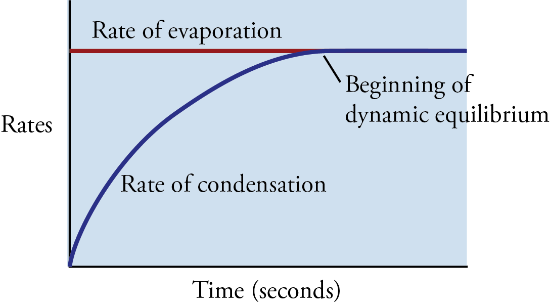
Graph of the changes in the rate of evaporation and the rate of condensation with time as they approach dynamic equilibrium
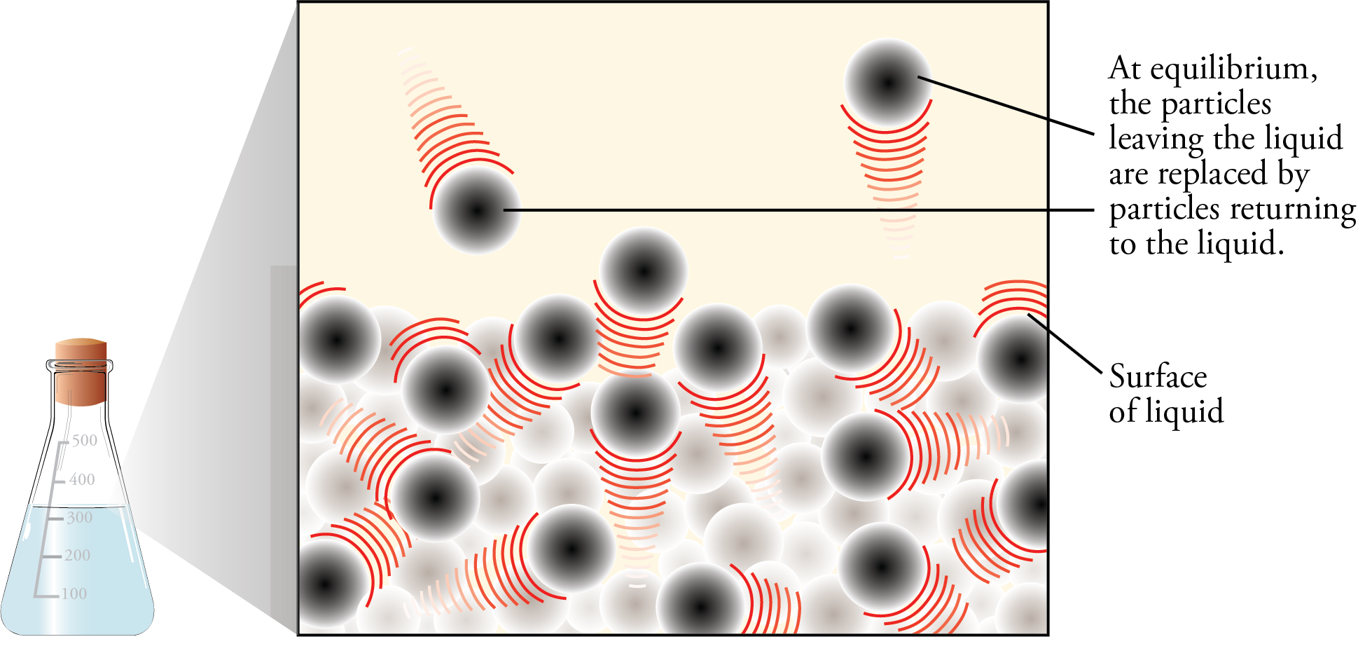
Evaporation and Condensation
Now let’s look at what happens for solutions instead of pure liquids. There are three general types of solutions. The first type is a solution of a nonvolatile, nonelectrolyte. An example is sugar in water. Nonelectrolytes dissolve as uncharged molecules and thus do not cause water to conduct electricity. Water soluble molecular compounds other than the acids and bases are generally nonelectrolytes (e.g. glucose or sucrose).
The addition of the nonvolatile, nonelectrolyte solute causes the vapor pressure of the solution to decrease. There are two reasons for this. The first is that the nonvolatile solute does not contribute to the overall vapor pressure, and the second reason is that the nonelectrolyte particles take some of the positions at the surface of the liquid, decreasing the number of solvent particles at the surface and decreasing the rate of evaporation. As the concentration of the solute increases, the effective surface area for the volatile solvent decreases. Because the rate of evaporation is lower, a lower rate of condensation is necessary to get to the stage where the two rates are equal. A lower concentration of vapor and therefore a lower vapor pressure would be necessary to reach this lower rate of condensation. If the solute-solvent attractions are the same strength as the solvent-solvent attractions, the following equation describes the vapor pressure of the solution.
PA = XAPA°
PA = the partial pressure of gas A in the solution
XA = the mole fraction for gas A
PA° = the vapor pressure of pure A
A solution for which this equation correctly predicts the vapor pressure is called an ideal solution
Boiling Point Elevation
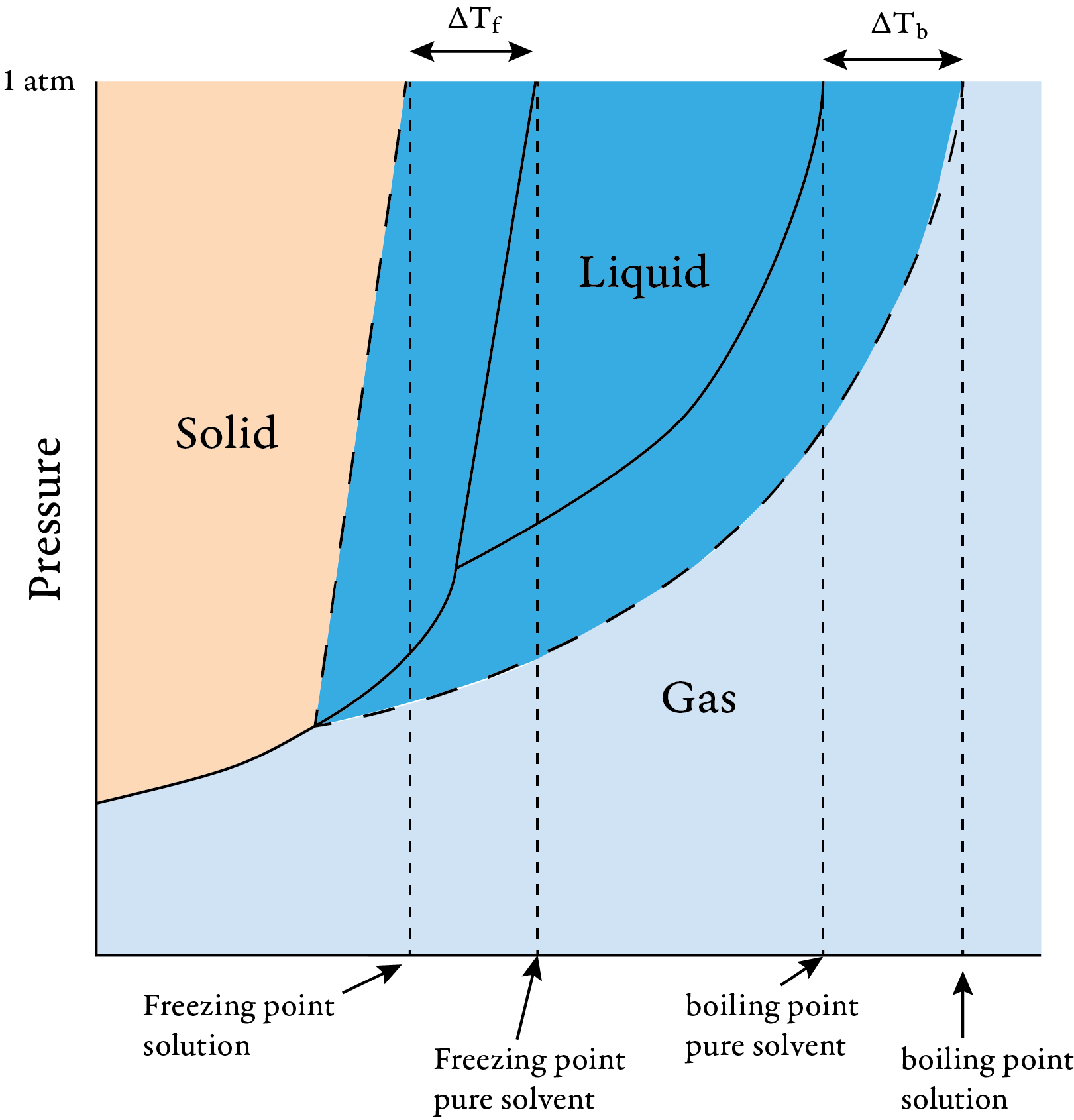
The lowering of the vapor pressure of the solution leads to an increase in the boiling point of the solution. An increase in the concentration of the nonvolatile, nonelectrolyte solute leads to a decrease in the equilibrium vapor pressure at a given temperature. For bubbles to form and thus for boiling to begin, the pressure in the bubble (the equilibrium vapor pressure) must be equal to the external pressure. Thus, a higher temperature is required to raise the vapor pressure up to being equal to the external pressure.
ΔTb = the change in the boiling point temperature
ΔTb is proportional to the concentration of solute
ΔTb = kbm
kb = the boiling point constant
m = molality = moles of solute/kg solvent
Tb,solution = Tb,pure solvent + ΔTb
The boiling point constant is a value that is unique to the solvent and determined experimentally
Exercise 1: Calculate the approximate boiling point of a solution that contains 1.5 g of the nonelectrolyte glycerin, C3H5(OH)3, in 30 g of water. (The boiling point constant for water is 0.512 °C/m. Assume that the glycerin is nonvolatile and that the solution is ideal.)
The next type of solution that we will consider is a solution of a nonvolatile electrolyte. An electrolyte is a solute that forms ions when it is added to water. The charged ions cause the water to conduct electricity. An example is the solution of sodium chloride in water. A strong electrolyte goes completely to ions completely when added to water. Water soluble ionic compounds and strong acids (HCl, HBr, HI, HNO3, H2SO4, HClO4) are strong electrolytes. Weak electrolytes ionize incompletely in water. Weak acids and uncharged bases, such as ammonia, are weak electrolytes.
For each mole of solute added to the solvent, an electrolyte yields more than one mole of particles in solution. Thus, an electrolyte has a greater effect on the colligative properties than a nonelectrolyte. For example, a 1 M solution of the nonelectrolyte glucose, C6H12O6, has 1 M glucose particles. A 1 M solution of the strong electrolyte sodium chloride, NaCl, has closer to 2 M particles. The greater number of particles in solution leads to a greater decrease in the vapor pressure above the solution and a greater increase in boiling point. The approximate boiling point elevation above a solution of a nonvolatile electrolyte can be calculated from the following equation.
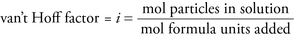
ΔTb = i kbm
i = van't Hoff factor
The van't Hoff factor accounts for this greater effect on colligative properties by electrolyte solutes.
The van't Hoff factor is an experimental quantity. It is 1 for nonelectrolytes and approximately equal to the number of ions per formula unit for ionic compounds. The formation of ion pairs in solution makes the van't Hoff factor somewhat less than the number of ions per formula unit. An ion pair is a combination of a cation and anion in solution that for a time acts as one particle. The higher the charges on the ions, the more ion pairs exist and the lower the van't Hoff factor. The more dilute the solution, the fewer the ion pairs and the closer the van't Hoff factor approaches the number of ions per formula unit.
van't Hoff factors at various concentrations
Electrolyte
0.001 m
0.01 m
0.1 m
NaCl
1.97
1.94
1.87
MgSO4
1.82
1.53
1.21
K2SO4
2.84
2.69
2.32
For solutions of two volatile, nonelectrolyte components, both components contribute to the total vapor pressure. An example would be alcohol and water. For an ideal solution, the total pressure can be calculated from the following formula. It is called Raoult's Law.
Ptotal = PA + PB = XAPA° + XBPA°
There are two types of deviations from ideal behavior. When the actual pressure is greater than the total pressure calculated from the above equation, we have positive deviation from Raoult's Law. This happens when the solute-solvent attractions are weaker than the separate solute-solute and solvent-solvent attractions. The solution cools as it forms because of the decrease in stability. Ethanol dissolving in water is an example.
When the actual pressure is less than the pressure calculated from the above equation, we have negative deviation from Raoult's Law. This happens when the solute-solvent attractions are stronger than the separate solute-solute and solvent-solvent attractions. The temperature rises as the solution forms due to the increase in stability. An example is formic acid dissolving in water.
Freezing point depression
The addition of a nonvolatile solute lowers the freezing point of a solution compared to that of the pure solvent. As the concentration of solute particles increases, it becomes more difficult for the solvent particles to find positions in the crystal lattice. Thus, the particles must move more slowly to solidify, and the freezing point decreases.
Another way to explain this is to recognize that the freezing point is the temperature where the vapor pressure of the liquid and the solid are equal. The following phase diagram shows that the temperature at which liquid and solid are in equilibrium is lower for a solution of a nonvolatile solute than for the pure solvent.
Phase diagram for pure solvent and solution
Calculations involving changes in freezing point can be done with an equation that is similar to that used for boiling point elevation. Freezing point constants and van't Hoff factors can be determined from tables.
ΔTf = the change in the freezing point temperature
ΔTf = kfm
kf = the freezing point constant
m = molality = moles of solute/kg solvent
Tf,solution = Tf,pure solvent + ΔTf
Exercise 2: What is the freezing point of a 0.01 m water solution of potassium sulfate? (The freezing point constant for water is -1.86 °C/m.